rRegressor Package

Celline Williem 120040005 Darren Boesono 120040022 Jefferson Joseph 120040023

rRegressor is a package containing several flexible and simple regression models for supervised learning. With rRegressor, you can easily fit linear, polynomial, ridge, lasso, and k-nearest neighbor regression models, as well as generate predictions and calculate Mean Squared Errors (MSE). This package also contains functions to compare regression models based on their MSE. The package also provides functions to plot the correlation between actual value and predicted value and plot the correlation between all variables of the data.

rRegressor is built with efficiency and flexibility in mind, allowing you to fit models with custom parameters. With its clear and concise documentation and intuitive API, rRegressor is designed to be user-friendly and accessible to all levels of R users. Whether you’re working on a small-scale project or a large-scale data analysis, rRegressor provides the tools you need to get the job done quickly and accurately. We hope that this vignette will help you get started with rRegressor and unleash the full power of regression analysis in R.

Package Installation

To install rRegressor, you can use the install.packages() function in R. However, since the package is in tar.gz file format, you will need to specify the path to the file using the repos = NULL argument. Here’s an example of how to install rRegressor:

install.packages("/path/to/rRegressor_0.1.0.tar.gz", repos = NULL, type = "source")

Note that you will need to replace “/path/to/” with the actual path to the rRegressor package on your local machine.

Load Package

To use rRegressor, you first need to load the library into your R session using the library() function. Here’s an example:

library(rRegressor)

Once you’ve loaded the library, you can start using the functions it provides. In the next section, we’ll take a closer look at the various regression functions that rRegressor provides, and how to use them to fit and evaluate regression models.

Load dataset

One of the datasets included in rRegressor is the Boston dataset, which contains information about housing values in suburbs of Boston. To load this dataset, you can simply call the Boston function in R:

data("boston_df")

This will load the Boston dataset into your R session as a data frame named boston_df.

The Boston dataset contains the following variables:

crim: per capita crime rate by town
zn: proportion of residential land zoned for lots over 25,000 sq.ft.
indus: proportion of non-retail business acres per town
chas: Charles River dummy variable (1 if tract bounds river; 0 otherwise)
nox: nitric oxides concentration (parts per 10 million)
rm: average number of rooms per dwelling
age: proportion of owner-occupied units built prior to 1940
dis: weighted distances to five Boston employment centers
rad: index of accessibility to radial highways
tax: full-value property-tax rate per $10,000
ptratio: pupil-teacher ratio by town
black: 1000(Bk - 0.63)^2 where Bk is the proportion of blacks by town
lstat: lower status of the population (percent)
medv: median value of owner-occupied homes in $1000s

Here’s an example for using the dataset:

head(boston_df)

##      crim zn indus chas   nox    rm  age    dis rad tax ptratio  black lstat
## 1 0.00632 18  2.31    0 0.538 6.575 65.2 4.0900   1 296    15.3 396.90  4.98
## 2 0.02731  0  7.07    0 0.469 6.421 78.9 4.9671   2 242    17.8 396.90  9.14
## 3 0.02729  0  7.07    0 0.469 7.185 61.1 4.9671   2 242    17.8 392.83  4.03
## 4 0.03237  0  2.18    0 0.458 6.998 45.8 6.0622   3 222    18.7 394.63  2.94
## 5 0.06905  0  2.18    0 0.458 7.147 54.2 6.0622   3 222    18.7 396.90  5.33
## 6 0.02985  0  2.18    0 0.458 6.430 58.7 6.0622   3 222    18.7 394.12  5.21
##   medv
## 1 24.0
## 2 21.6
## 3 34.7
## 4 33.4
## 5 36.2
## 6 28.7

Data Exploration using Correlation Matrix

Create Correlation Matrix using `plot_correlation_matrix()`

The plot_correlation_matrix function in rRegressor is a useful tool for exploring the pairwise correlations between variables in a dataset. By visualizing the correlation matrix using a color-coded plot, you can quickly identify which variables are positively or negatively correlated, and to what degree.

Understanding the correlations between variables in your dataset can help you to identify potential relationships that may be useful for building regression models. Before fitting and predicting regression models, it’s often a good idea to explore the correlations in your dataset using a function like plot_correlation_matrix. This can help you to identify potential multicollinearity issues (where two or more variables are highly correlated), which can make it difficult to interpret the coefficients of your regression models.

Parameters

The plot_correlation_matrix function takes three parameters:

data: A data frame containing the variables to plot correlations for.
title: The title to use for the plot.
size_coercoef: The size of the correlation coefficients displayed in the plot. By default, this is set to 0.5.

Loading the ‘corrplot’ Package

The plot_correlation_matrix function relies on the corrplot package to generate the correlation matrix plot. If the corrplot package is not already installed, the function will automatically install it using the install.packages()

Example

Here’s an example of how to use the plot_correlation_matrix() with the Boston dataset:

boston_df %>%  
  plot_correlation_matrix(.,title = "Boston Housing Dataset Correlation Matrix", 
                          size_coercoef = 0.7)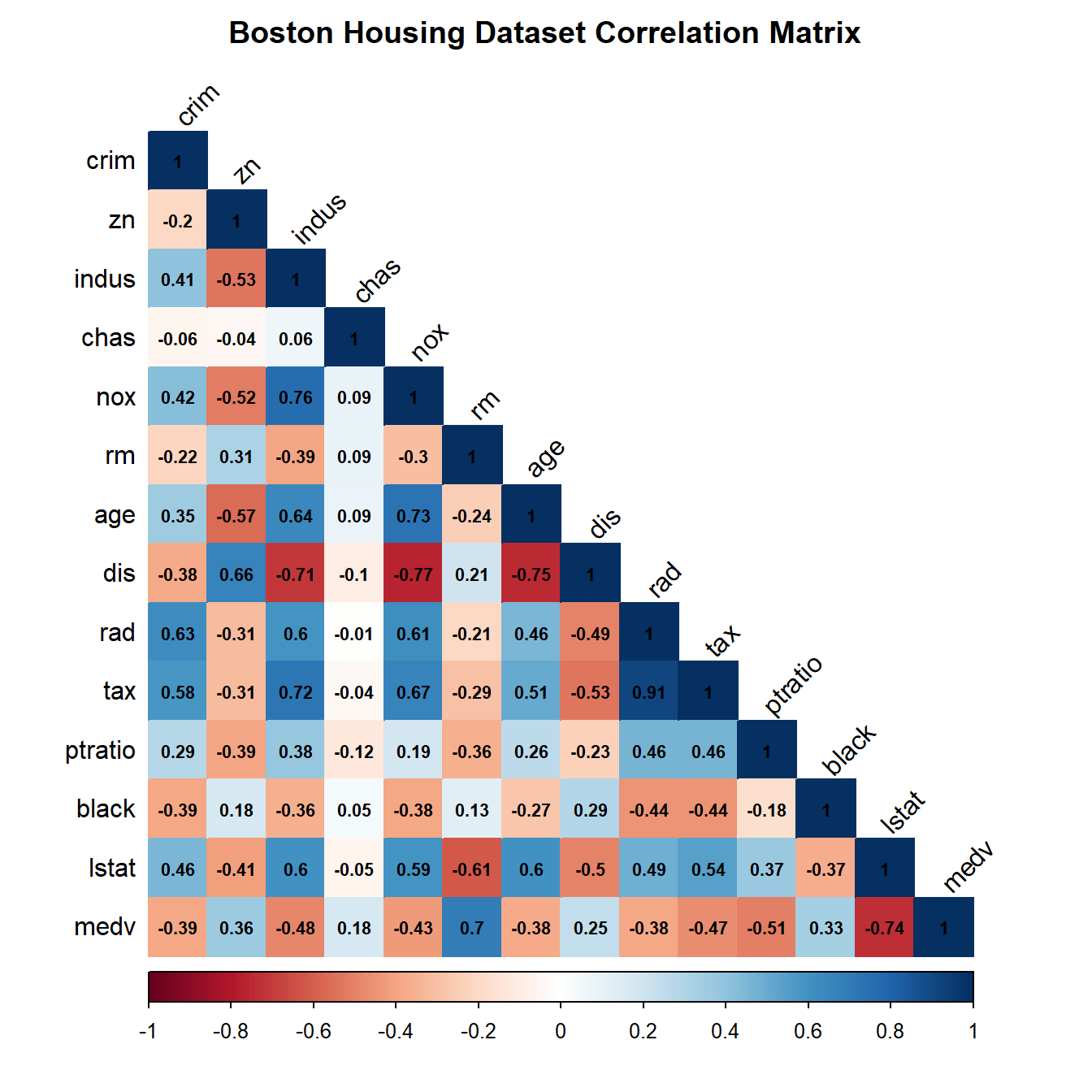

This will generate a color-coded plot of the correlation matrix for the Boston dataset, with the correlation coefficients displayed in the lower triangle of the plot. You can use this plot to explore the relationships between the variables in the dataset and identify potential predictors for your regression models.

Regression Models

1. Linear Regression

Linear regression is a commonly used statistical technique for modeling the relationship between a response variable and one or more predictor variables. In simple linear regression, we model the relationship between a single predictor variable and a response variable using the following equation: \[y = \beta_0 + \beta_1 x + \epsilon\]

where $y$ is the response variable, $x_1$ is the predictor variable, $\beta_0$ is the intercept term, $\beta_1$ is the slope coefficient, and $\epsilon$ is the error term. The goal of linear regression is to estimate the values of the intercept and slope coefficients that minimize the sum of squared errors between the predicted values and the actual values of the response variable.

In multiple linear regression, we extend this concept to include multiple predictor variables, using the following equation: \[y = \beta_0 + \beta_1 x_1 + \beta_2 x_2 + \cdots + \beta_p x_p + \epsilon\]

where $y$ is the response variable, $x_1, x_2, \dots, x_p$ are the predictor variables, $\beta_0$ is the intercept term, $\beta_1, \beta_2, \dots, \beta_p$ are the slope coefficients, and $\epsilon$ is the error term.

Fit a Linear Regression Model with `fit_linear_regression()`

The fit_linear_regression function in rRegressor is a tool for fitting a simple linear regression model to a dataset. It uses the normal equation to calculate the coefficients that minimize the sum of squared errors between the predicted values and the actual values of the response variable. The normal equation is given by: \[\beta = (X^TX)^{-1}X^Ty\]

where $\beta$ is the vector of slope coefficients, $X$ is the design matrix consisting of the predictor variables (with an optional intercept term), and $y$ is the vector of response variable values.

After calculating the slope coefficients, fit_linear_regression() uses them to calculate the fitted values for the response variable, using the equation: \[\hat{y} = X\beta\]

where $\hat{y}$ is the vector of fitted values for the response variable, $X$ is the design matrix consisting of the predictor variables (with an optional intercept term), and $\beta$ is the vector of slope coefficients.

Parameters

The fit_linear_regression function takes four parameters:

data: A data frame containing the predictor and response variables.
x_vars: A character vector of variable names to be used as predictors.
y_var: A character string of the variable name to be used as the response variable.
intercept: A logical value indicating whether to include an intercept term in the model. The default value is TRUE.

Output

The fit_linear_regression function returns a list containing the following elements:

model: A list containing the slope coefficients and residuals for the linear regression model.
fitted_values: A vector of the fitted values for the response variable.

Example

Here’s an example of how to use the fit_linear_regression function with the Boston dataset:

# Fit a linear regression model
lm_fit <- boston_df[1:10,] %>% fit_linear_regression(., x_vars = c("age", "rm", "lstat"), 
                                                     y_var = "medv")

# Display the model object
lm_fit$model

## $coefficients
##              medv
##       -53.6997418
## age    -0.1332504
## rm     13.2566640
## lstat   0.3618399
## 
## $residuals
##          medv
## 1  -2.5768622
## 2  -2.6150599
## 3  -0.1660058
## 4  -0.6313349
## 5   0.4479279
## 6   3.0960035
## 7   1.2774826
## 8   4.8557381
## 9  -1.9533649
## 10 -1.7345244

# Display the fitted values
lm_fit$fitted_values

##        medv
## 1  26.57686
## 2  24.21506
## 3  34.86601
## 4  34.03133
## 5  35.75207
## 6  25.60400
## 7  21.62252
## 8  22.24426
## 9  18.45336
## 10 20.63452

This shows that the fit_linear_regression function has successfully fit a linear regression model to the Boston dataset, with age, rm, and lstat as the predictor variable and medv as the response variable. The model object and fitted values are displayed as output in the R Markdown document.

Predict a Linear Regression Model with `predict_linear_regression()`

The predict_linear_regression function uses the fitted model obtained from the fit_linear_regression function to predict the response variable using the predictor variables in the data parameter. The predicted values are calculated using the following equation: \[\hat{y} = X\beta\]

where $\hat{y}$ is the vector of predicted values for the response variable, $X$ is the design matrix consisting of the predictor variables (with an optional intercept term), and $\beta$ is the vector of slope coefficients obtained from the ‘lm_fit’ parameter.

Parameters

data: a data frame containing the feature variables.
lm_fit: a list containing the model object and fitted values obtained from the fit_linear_regression function.
x_vars: a character vector of variable names to be used as predictors.
intercept: a logical value indicating whether to include an intercept term in the model.

Output

The function returns a numeric vector of predicted values for the response variable.

Example

Here’s an example of how to use the predict_linear_regression function with the Boston dataset:

# Fit and predict a linear regression model
lm_pred = boston_df[1:10,] %>% fit_linear_regression(.,
                                                     x_vars = c("age","rm","lstat"), 
                                                     y_var = "medv") %>% 
  predict_linear_regression(data = boston_df[40:50,],
                            lm_fit = .,
                            x_vars = c("age","rm","lstat"))

#Display the predicted values
lm_pred

##        medv
## 40 32.38625
## 41 38.02615
## 42 37.41275
## 43 29.30346
## 44 30.46336
## 45 24.88051
## 46 20.81515
## 47 23.68611
## 48 21.64763
## 49 16.32251
## 50 18.16437

2. Ridge Regression

Ridge regression is a regularized version of linear regression that shrinks the regression coefficients towards zero to avoid overfitting. The objective function of Ridge regression is as follows: \[\min_{\beta_0, \beta_1, ..., \beta_p} \sum_{i=1}^{n} (y_i - \beta_0 - \sum_{j=1}^{p} \beta_j x_{ij})^2 + \lambda \sum_{j=1}^{p} \beta_j^2\]

where $\beta_0$ is the intercept term, $\beta_1, \beta_2, ..., \beta_p$ are the slope coefficients, $x_{ij}$ is the $i$th observation of the $j$th predictor variable, $y_i$ is the $i$th observation of the response variable, $\lambda$ is the regularization parameter, and $p$ is the number of predictor variables.

Fit a Ridge Regression Model with `fit_ridge_regression()`

The fit_ridge_regression function uses the Ridge regression formula to calculate the beta coefficients for the given data. The beta coefficients are calculated using the following equation: \[\hat{\beta}_{ridge} = (X^TX + \lambda I_p)^{-1}X^Ty\]

where $\hat{\beta}$ is the vector of beta coefficients, $X$ is the design matrix consisting of the predictor variables (with an optional intercept term), $y$ is the vector of response variable observations, $\lambda$ is the regularization parameter, and $I$ is the identity matrix.

After calculating the beta coefficients, fit_ridge_regression() uses them to calculate the fitted values for the response variable, using the equation: \[\hat{y} = X\beta\]

Parameters

data: a data frame containing the feature and label variables.
x_vars: a character vector of variable names to be used as predictors.
y_var: a character string of the variable name to be used as the response variable.
lambda: the value of the regularization parameter.
intercept: a logical value indicating whether to include an intercept term in the model.

Output

The function returns a list containing the model object and fitted values.

Example

Here’s an example of how to use the fit_ridge_regression():

# Fit a Ridge regression model using the 'rm' (number of rooms) and 'lstat' (percent of lower status of the population) variables as predictors
ridge_fit <- boston_df[1:10,] %>%  fit_ridge_regression(., 
                                                        x_vars = c("rm", "lstat"), 
                                                        y_var = "medv", 
                                                        lambda = 0.1)

# Display the model object
ridge_fit$model

## $coefficients
##             medv
##       -6.8269184
## rm     5.6575651
## lstat -0.2937717
## 
## $residuals
##          medv
## 1  -4.9085891
## 2  -5.2152339
## 3   2.0612130
## 4   1.4989666
## 5   4.1581037
## 6   0.6793253
## 7  -0.6347809
## 8   4.6341544
## 9   0.2617558
## 10 -3.2176067

# Display the fitted values
ridge_fit$fitted_values

##        medv
## 1  28.90859
## 2  26.81523
## 3  32.63879
## 4  31.90103
## 5  32.04190
## 6  28.02067
## 7  23.53478
## 8  22.46585
## 9  16.23824
## 10 22.11761

Predict a Ridge Regression Model with `predict_ridge_regression()`

The formula for predicting the response variable for new observations using the Ridge regression model is: \[\hat{y} = X_{new}\hat{\beta}\]

where $\hat{y}$ is the predicted response variable for new observations, $X_{new}$ is the matrix of predictor variables for the new observations, and $\hat{\beta}$ is the estimated vector of coefficients obtained from the Ridge regression model.

Parameters

data: a data frame containing the feature variables
ridge_fit: a list containing the model object and fitted values obtained from the fit_ridge_regression() function
x_vars: a character vector of variable names to be used as predictors

Output

The predict_ridge_regression() function returns a numeric vector of predicted values.

Example

Here’s an example of how to use the fit_ridge_regression():

# Predict the median value using the Ridge regression model
ridge_pred <- boston_df %>% fit_ridge_regression(., x_vars = c("rm", "lstat"), 
                                                 y_var = "medv", lambda = 0.1) %>% 
  predict_ridge_regression(data = boston_df,.,x_vars = c("rm","lstat"))

# Print the first six predicted values
head(ridge_pred)

##          medv
## [1,] 28.94331
## [2,] 25.48537
## [3,] 32.65640
## [4,] 32.40621
## [5,] 31.62728
## [6,] 28.05801

3. Lasso Regression

Lasso (Least Absolute Shrinkage and Selection Operator) regression is a type of linear regression that adds a penalty term to the objective function to shrink the coefficients of the model towards zero, effectively performing feature selection. It is particularly useful in high-dimensional datasets, where the number of features is much larger than the number of observations.

The objective function for Lasso regression is given by: \[\text{minimize } \frac{1}{2n} \sum_{i=1}^n (y_i - \beta_0 - \sum_{j=1}^p x_{ij}\beta_j)^2 + \lambda\sum_{j=1}^p |\beta_j|\]

Where $n$ is the number of observations, $p$ is the number of features, $y_i$ is the target variable for the $i$th observation, $x_{ij}$ is the value of the $j$th feature for the $i$th observation, $\beta_0$ is the intercept term, $\beta_j$ is the coefficient for the $j$th feature, and $\lambda$ is the regularization parameter.

Fit a Lasso Regression Model with `fit_lasso_regression()`

To minimize the objective function, we can use the coordinate descent algorithm. The basic idea of coordinate descent is to update one coordinate (i.e., one coefficient) at a time, while holding all other coordinates fixed. At each iteration, we choose the coordinate with the steepest descent and update it using a closed-form solution that involves solving a univariate optimization problem. We repeat this process until convergence. This algorithm is computationally efficient for Lasso regression, because the penalty term has a special structure that allows us to solve the univariate optimization problem analytically using a soft thresholding operator.

The update rule for the coefficients in Lasso regression using coordinate descent is given by: \[\beta_j = \text{sign}\left(\sum_{i=1}^{n}x_{ij}(y_i - \beta_0 - \sum_{k \neq j}x_{ik}\beta_k)\right)\max{|\sum_{i=1}^{n}x_{ij}(y_i - \beta_0 - \sum_{k \neq j}x_{ik}\beta_k)| - \lambda, 0} ,/, \sum_{i=1}^{n}x_{ij}^2\] where:

$\beta_j^{new}$: The updated value of the $j$-th coefficient.
$\beta_j$: The current value of the $j$-th coefficient.
$x_j$: The $j$-th predictor variable.
$r_j$: The residual error of the regression model when the $j$-th predictor variable is removed from the model.
$z_j$: The “squared length” of the $j$-th predictor variable.
$\lambda$: The regularization parameter controlling the strength of the L1 penalty. A larger value of - $\lambda$ leads to stronger shrinkage of the coefficient estimates.
$\alpha$: The mixing parameter controlling the balance between the L1 and L2 penalties. A value of $\alpha=1$ corresponds to pure Lasso regression, while a value of $\alpha=0$ corresponds to pure Ridge regression.
$n$: The number of observations in the dataset.

The update rule for the intercept in Lasso regression using coordinate descent is given by: \[\beta_0 = \frac{1}{n} \sum_{i=1}^{n}(y_i - \sum_{j=1}^{p}\beta_j x_{ij})\]

where $n$ is the number of observations, $p$ is the number of predictors, $y_i$ is the response variable for the $i$th observation, $x_{ij}$ is the value of the $j$th predictor for the $i$th observation, and $\beta_j$ is the coefficient of the $j$th predictor in the model. The update rule for the intercept simply sets it equal to the mean of the residuals of the current model, which is the difference between the actual response values and the predicted response values using the current coefficients.

Parameters

The fit_lasso_regression() function fits a Lasso regression to a given dataset using coordinate descent. It takes in the following parameters:

data: a data frame containing the predictor and response variables.
x_vars: a character vector of column names corresponding to the predictor variables.
y_var: a character string of the column name corresponding to the response variable.
lambda: the regularization parameter.
alpha: the mixing parameter between L1 and L2 penalties (default = 1).
max_iter: the maximum number of iterations for the coordinate descent algorithm (default = 1000).
tol: the convergence threshold for the coordinate descent algorithm (default = 1e-4).

Output

The fit_lasso_regression() function returns a list containing the fitted coefficients and the intercept.

Example

Here’s an example of using fit_lasso_regression() function with the Boston Housing dataset:

# Fit the Lasso regression using the function
fit <- boston_df %>%  fit_lasso_regression(., x_vars = colnames(boston_df)[1:13], 
                                           y_var = "medv", lambda = 0.1)

# Print the coefficients
fit$coefficients

##  [1] -0.92898269  1.08262512  0.14082789  0.68243539 -2.05863101  2.67689637
##  [7]  0.01948712 -3.10714827  2.66434285 -2.07840300 -2.06257282  0.85008881
## [13] -3.74734521

#Print the intercept
fit$intercept

## [1] 22.53281

Predict a Lasso Regression Model with `predict_ridge_regression()`

The fit_lasso_regression() function uses coordinate descent to solve for the coefficients and intercept that minimize this objective function. Once these coefficients and intercept have been determined, they can be used to make predictions on new data using the predict_lasso_regression() function.

The predicted response variable values for new data can be calculated as:

\[ \hat{y} = \beta_0 + \sum\limits_{j=1}^{p} x_j \beta_j \]

where:

$\hat{y}$ is the predicted response variable value for a new observation
$x_j$ is the value of predictor $j$ for the new observation
$\beta_0$ is the intercept term
$\beta_j$ is the coefficient for predictor $j$

Parameters

The predict_lasso_regression() function takes the following parameters:

fit: a list containing the fitted coefficients and intercept from the fit_lasso_regression function
new_data: a data frame containing the predictor variables for which predictions are to be made
x_vars: a character vector of column names corresponding to the predictor variables

Output

The predict_lasso_regression() function returns a numeric vector of predicted response variable values.

Example

Here’s an example of using predict_lasso_regression() function with the Boston Housing dataset:

# Make predictions using the fitted model
lasso_pred <- boston_df %>% fit_lasso_regression(., x_vars = colnames(boston_df)[1:13], 
                                                 y_var = "medv", lambda = 0.1) %>% 
  predict_lasso_regression(fit = ., new_data = boston_df, 
                           x_vars = colnames(boston_df)[1:13])

# Print the first 10 predicted values
head(lasso_pred, n = 10)

##           [,1]
##  [1,] 30.00417
##  [2,] 25.02554
##  [3,] 30.56760
##  [4,] 28.60708
##  [5,] 27.94357
##  [6,] 25.25631
##  [7,] 23.00170
##  [8,] 19.53587
##  [9,] 11.52348
## [10,] 18.92013

4. Polynomial Regression

Polynomial regression is a type of regression analysis in which the relationship between the independent variable X and the dependent variable Y is modeled as an nth degree polynomial. The model equation can be written as: \[y = \beta_0 + \beta_1 x + \beta_2 x^2 + ... + \beta_k x^k + \epsilon\] where:

$y$ is the response variable
$x$ is the predictor variable
$k$ is the degree of the polynomial
$\beta_0, \beta_1, \beta_2, ..., \beta_k$ are the coefficients to be estimated
$\epsilon$ is the error term.

Fit a Polynomial Regression Model with `fit_polynomial_regression()`

The fit_polynomial_regression function fits a polynomial regression model to a dataset using the normal equation. To obtain the coefficients in polynomial regression, we need to use the Normal Equation, which is derived by minimizing the sum of squared errors between the predicted values and actual values. The Normal Equation is given by: \[\hat{\beta} = (X^TX)^{-1}X^Ty\]

where $\hat{\beta}$ is a vector of the estimated coefficients, $X$ is the design matrix with polynomial terms and interaction terms, $y$ is the vector of response variables.

The solution to the Normal Equation gives us the optimal values of the coefficients that minimize the sum of squared errors between the predicted values and actual values. The solution is found by taking the inverse of the matrix $X^TX$ and multiplying it by the matrix product $X^Ty$.

In the fit_polynomial_regression() function, we first create the design matrix with polynomial terms and interaction terms using the model.matrix() function. We then use the Normal Equation to obtain the optimal values of the coefficients by solving the equation: $X^TX \hat{\beta} = X^Ty$ for $\hat{\beta}$.

Once we have the optimal values of the coefficients, we return them along with the design matrix in a list.

Parameters

The function takes the following arguments:

data: a data frame containing the predictor and response variables
x_vars: a character vector of column names corresponding to the predictor variables
y_var: a character string of the column name corresponding to the response variable
degree: the degree of the polynomial (default = 2)

Output

The function returns a list containing the fitted coefficients and the design matrix. The design matrix is a matrix of predictor variables, where each column represents a polynomial term or an interaction term. The first column of the design matrix is a column of ones, representing the intercept term.

Example

Here’s an example of using the fit_polynomial_regression() function with the Boston dataset:

# Fit a polynomial regression model
poly_fit <- boston_df %>% fit_polynomial_regression(., x_vars = c("age", "rm", "lstat"), 
                                                    y_var = "medv", degree = 2)

# Print the fitted coefficients
poly_fit$coefficients

##                     [,1]
## (Intercept) -78.71823177
## age           0.65961841
## rm           15.97999835
## lstat         3.06941245
## age:rm       -0.08331668
## age:lstat    -0.01197715
## rm:lstat     -0.46956897

#Print the first 10 design matrix
head(poly_fit$design_matrix, n = 10)

##    (Intercept)   age    rm lstat   age:rm age:lstat  rm:lstat
## 1            1  65.2 6.575  4.98 428.6900   324.696  32.74350
## 2            1  78.9 6.421  9.14 506.6169   721.146  58.68794
## 3            1  61.1 7.185  4.03 439.0035   246.233  28.95555
## 4            1  45.8 6.998  2.94 320.5084   134.652  20.57412
## 5            1  54.2 7.147  5.33 387.3674   288.886  38.09351
## 6            1  58.7 6.430  5.21 377.4410   305.827  33.50030
## 7            1  66.6 6.012 12.43 400.3992   827.838  74.72916
## 8            1  96.1 6.172 19.15 593.1292  1840.315 118.19380
## 9            1 100.0 5.631 29.93 563.1000  2993.000 168.53583
## 10           1  85.9 6.004 17.10 515.7436  1468.890 102.66840

Predict a Polynomial Regression Model with `predict_polynomial_regression()`

The predict_polynomial_regression() function is used to predict the response variable using the fitted polynomial regression model. The function takes the fitted model object, new predictor variable values, and the degree of the polynomial as inputs, and returns a vector of predicted response variable values.

The equation for making predictions using a polynomial regression model is as follows: \[\hat{y} = X_{new} \hat{\beta}\] where $\hat{y}$ is the predicted response variable values, $X_{new}$ is the design matrix for the new predictor variable values, and $\hat{\beta}$ is the vector of fitted coefficients.

Parameters

model: A list containing the fitted coefficients and the design matrix of the Polynomial Regression model
new_data: A data frame containing the new predictor variable values
x_vars: A character vector of column names corresponding to the predictor variables
degree: The degree of the polynomial (default = 2)

Output

The function gives an output in a vector of predicted response variable values

Example

Here’s an example of using the predict_polynomial_regression() function with the Boston dataset:

# Create new data with lstat and age values
new_data <- data.frame(lstat = c(5.0, 10.0), age = c(50, 60))

# Predict the response variable using the fitted model
predictions <- boston_df %>% fit_polynomial_regression(., x_vars = c("lstat", "age"), 
                                                       y_var = "medv", degree = 2) %>% 
  predict_polynomial_regression(model = ., new_data = new_data, 
                                x_vars = c("lstat", "age"), degree = 2)

# Print the predictions
predictions

##       [,1]
## 1 30.13090
## 2 24.61769

5. K-Nearest Neighbors Regression

K-Nearest Neighbor (KNN) Regression is a non-parametric method used for regression tasks. The KNN regression algorithm works by finding the K-nearest neighbors in the training set to a given new data point, and then estimating the response variable for that new data point based on the mean of the response variable of its K-nearest neighbors.

To find the K-nearest neighbors, the algorithm computes the Euclidean distance between each point in the training set and the new data point. The Euclidean distance is a measure of the distance between two points in a Euclidean space, and it is calculated as the square root of the sum of the squared differences between each coordinate.

Once the K-nearest neighbors are identified, the algorithm estimates the response variable for the new data point as the mean of the response variable of its K-nearest neighbors.

Predict a K-Nearest Neighbors Regression Model with `predict_knn_regression()`

The KNN regression model can be represented by the following equation: \[\hat{y}(x) = \frac{1}{k}\sum_{i\in N_k(x)} y_i\]

where $\hat{y}(x)$ is the predicted response variable for a new data point $x$, $N_k(x)$ is the set of $k$ nearest neighbors of $x$ in the training data, and $y_i$ is the response variable value for the $i$-th training data point.

Parameters

The function takes the following parameters:

data: A data frame containing the predictor and response variables used to fit the KNN regression model.
x_vars: A character vector of column names corresponding to the predictor variables.
y_var: A character string of the column name corresponding to the response variable.
new_data: A data frame containing the new predictor variable values.
k: The number of nearest neighbors to consider (default = 5).

Output

The output of the function is a vector of predicted response variable values for the new data.

Example

Here’s an example of using the predict_knn_regression() function with the Boston dataset:

# Split the data into training and test sets
set.seed(123)
train_indices <- sample(1:nrow(boston_df), 0.7 * nrow(boston_df))
train_data <- boston_df[train_indices, ]
test_data <- boston_df[-train_indices, ]

# Make predictions using the KNN regression model
predictions <- train_data %>% predict_knn_regression(., x_vars=colnames(train_data)[-14], 
                                                     y_var="medv", new_data=test_data[, -14], k=5)

# The first 10 predicted values
head(predictions, n = 10)

##     1     3     6     8     9    12    15    17    18    19 
## 21.56 22.62 25.16 17.28 16.74 20.80 30.18 30.20 21.18 18.66

Actual Values vs Predicted Values

The plot_y_actual_vs_predicted() function is a custom function that creates a scatterplot of the actual vs. predicted values of a response variable for a specified regression model from the rRegressor package. The function takes three arguments: y_actual, y_pred, and model_name.

Parameters

The parameters of the function includes:

y_actual: A numeric vector of the actual response variable values.
y_pred: A numeric vector of the predicted response variable values.
model_name: A character string representing the name of the regression model used for predictions.

Output

The function returns a scatterplot using the ggplot2 package and also includes a red dashed line representing the ideal 1:1 relationship between the actual and predicted values. The plot is titled “Actual vs. Predicted Values for model_name”.

Example 1: Linear Regression

In this example, we will use the plot_y_actual_vs_predicted() function using the linear regression as our regression model.

# Predict using the fitted model
predictions = boston_df %>% fit_linear_regression(., x_vars = c("age", "rm", "lstat"), y_var = "medv") %>% 
  predict_linear_regression(data = boston_df, lm_fit = .,x_vars = c("age", "rm", "lstat"))


# Create a scatterplot of actual vs. predicted values using the plot_y_actual_vs_predicted function
actual_vs_pred_plot <- plot_y_actual_vs_predicted(boston_df[["medv"]], predictions , "Linear Regression")

## Warning: package 'ggplot2' was built under R version 4.1.3

actual_vs_pred_plot

Example 2: Lasso Regression

In this example, we will use the plot_y_actual_vs_predicted() function using the Lasso Regression as our regression model.

# Make predictions using the fitted model
lasso_pred <- boston_df %>% fit_lasso_regression(., x_vars = colnames(boston_df)[1:13], y_var = "medv", lambda = 0.1) %>% 
  predict_lasso_regression(fit = ., new_data = boston_df, x_vars = colnames(boston_df)[1:13])

# Plot the actual vs. predicted values
lasso_plot <- plot_y_actual_vs_predicted(y_actual = boston_df[, "medv"], y_pred = predictions, model_name = "Lasso Regression")
print(lasso_plot)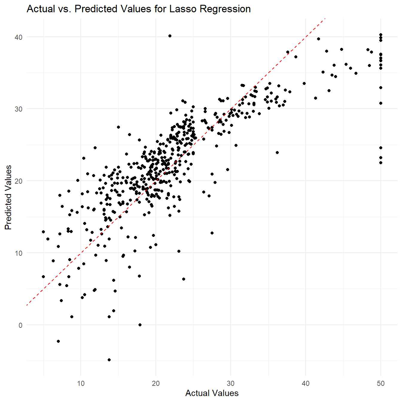

By visualizing the actual vs. predicted values, we can get a better understanding of how well our regression model is performing in predicting the response variable. The plot can help us assess if there are any systematic patterns in the residuals or if the model is capturing the overall trend in the data.

Calculate the Mean Squared Error (MSE)

Mean Squared Error (MSE) is a common metric used to measure the accuracy of a regression model. It measures the average squared differences between the predicted and actual values of the response variable. The MSE gives us an idea of how much the predicted values differ from the actual values. The MSE is calculated using the following formula: \[MSE = \frac{1}{n}\sum_{i=1}^{n}(y_i - \hat{y}_i)^2\] where $y_i$ is the actual value of the response variable, $\hat{y_i}$ is the predicted value of the response variable and $n$ is the number of observations. ### Calculate the MSE using calc_mse() function The calc_mse() function takes two arguments y and y_pred which are numeric vectors of actual response values and predicted response values respectively. The function checks that y and y_pred are numeric vectors of the same length and then calculates the mean squared error using the formula shown above. The function returns the calculated MSE.

Parameters

y: a numeric vector of actual response values.
y_pred: a numeric vector of predicted response values.

Output

The function returns a numeric value of the calculated mean squared error.

Example

Here’s an example of using the calc_mse() function:

# Split the data into training and test sets
set.seed(123)
train_indices <- sample(1:nrow(boston_df), 0.7 * nrow(boston_df))
train_data <- boston_df[train_indices, ]
test_data <- boston_df[-train_indices, ]

# Make predictions using the KNN regression model
predictions <- predict_knn_regression(train_data, x_vars=colnames(train_data)[-14], y_var="medv", new_data=test_data[, -14], k=5)

# Calculate the MSE
calc_mse(test_data[["medv"]], predictions)

## [1] 44.15632

Compare Regression Models

The compare_regression_models() function compares different regression models based on their Mean Squared Error(MSE). It fits linear regression, ridge regression, lasso regression, polynomial regression, and k-nearest neighbors (k-NN) regression models to the given dataset and calculates their MSE on new data.

Parameters

The parameters of the function includes:

data: A data frame containing the data to fit the models.
x_vars: A character vector of predictor variable names.
y_var: A character string of the response variable name.
new_data: A data frame containing the data for making predictions.
lambda: A numeric value for the ridge and lasso regularization parameter (default is 1).
alpha: A numeric value for the lasso mixing parameter (default is 1).
max_iter: A numeric value for the maximum number of iterations for lasso (default is 1000).
tol: A numeric value for the tolerance for lasso convergence (default is 1e-4).
degree: A numeric value for the polynomial regression degree (default is 2).
k: A numeric value for the number of neighbors for k-NN regression (default is 5).

Output

The function returns a data frame showing the models and their corresponding MSE values, sorted by the smallest MSE.

Example

Here’s an example of compare_regression_models() function:

#define the predictor variables and response variables
x_vars <- c("age", "rm", "tax", "lstat")
y_var <- "medv"

#Split the data into training and testing sets
set.seed(123)
train_indices <- sample(seq_len(nrow(boston_df)), size = 0.8 * nrow(boston_df))
train_data <- boston_df[train_indices, ]
test_data <- boston_df[-train_indices, ]

#Compare the regression models using the `compare_regression_models()` function
results <- train_data %>%
  compare_regression_models(
    x_vars = x_vars,
    y_var = y_var,
    new_data = test_data,
    lambda = 1,
    alpha = 1,
    max_iter = 1000,
    tol = 1e-4,
    degree = 2,
    k = 5
  )

#Display the result
results

##                   Model      MSE
## 4 Polynomial Regression 18.57330
## 1     Linear Regression 29.59409
## 2      Ridge Regression 29.59617
## 3      Lasso Regression 29.83161
## 5        kNN Regression 42.81067

Conclusion

Advantage of the package

rRegressor provides several advantages for users. Firstly, the package contains several useful regression functions, including polynomial regression, lasso regression, and KNN regression. These functions are commonly used in machine learning and statistical analysis, making the package useful for a wide range of users in academia and industry. Additionally, the package includes a function to calculate the mean squared error, which is a common metric used to evaluate the performance of regression models. This feature makes it easy for users to evaluate the accuracy of their models and make comparisons between different models. Another advantage of the package is its ability to compare multiple regression models using the compare_regression_models() function. This can help users determine which model performs the best and make informed decisions on which model to choose for their specific analysis. Overall, the package provides a comprehensive set of tools for users to perform various types of regression analysis and evaluate their model performance, while also prioritizing user experience and efficient computation.

Learned points from STA3005 course

The applications of STA3005 course materials in the process of creating an R package:

Chapter 5: Write examples for vignette using pipe operator %>%
Chapter 7: Visualization using ggplot2 for the plot_y_actual_vs_predicted() function
Chapter 8: Write R functions for the R package
Chapter 9: Build an R package, modify DESCRIPTION file, use roxygen, write vignettes, write automated tests

Regression Models for Supervised Learning

Package Installation

Load Package

Load dataset

Data Exploration using Correlation Matrix

Create Correlation Matrix using plot_correlation_matrix()

Parameters

Loading the ‘corrplot’ Package

Example

Regression Models

1. Linear Regression

Fit a Linear Regression Model with fit_linear_regression()

Parameters

Output

Example

Predict a Linear Regression Model with predict_linear_regression()

Parameters

Output

Example

2. Ridge Regression

Fit a Ridge Regression Model with fit_ridge_regression()

Parameters

Output

Example

Predict a Ridge Regression Model with predict_ridge_regression()

Parameters

Output

Example

3. Lasso Regression

Fit a Lasso Regression Model with fit_lasso_regression()

Parameters

Output

Example

Predict a Lasso Regression Model with predict_ridge_regression()

Parameters

Output

Example

4. Polynomial Regression

Fit a Polynomial Regression Model with fit_polynomial_regression()

Parameters

Output

Example

Predict a Polynomial Regression Model with predict_polynomial_regression()

Parameters

Output

Example

5. K-Nearest Neighbors Regression

Predict a K-Nearest Neighbors Regression Model with predict_knn_regression()

Parameters

Output

Example

Actual Values vs Predicted Values

Parameters

Output

Example 1: Linear Regression

Example 2: Lasso Regression

Calculate the Mean Squared Error (MSE)

Parameters

Output

Example

Compare Regression Models

Parameters

Output

Example

Conclusion

Advantage of the package

Learned points from STA3005 course

Create Correlation Matrix using `plot_correlation_matrix()`

Fit a Linear Regression Model with `fit_linear_regression()`

Predict a Linear Regression Model with `predict_linear_regression()`

Fit a Ridge Regression Model with `fit_ridge_regression()`

Predict a Ridge Regression Model with `predict_ridge_regression()`

Fit a Lasso Regression Model with `fit_lasso_regression()`

Predict a Lasso Regression Model with `predict_ridge_regression()`

Fit a Polynomial Regression Model with `fit_polynomial_regression()`

Predict a Polynomial Regression Model with `predict_polynomial_regression()`

Predict a K-Nearest Neighbors Regression Model with `predict_knn_regression()`